You can create your own pull-down list or combo box by using the data validation feature in Excel but the main problem is the list has to be in the same spreadsheet as the combo box that you want to use. What most of us will do is just create a list somewhere else in the same spreadsheet and then hide it either by hiding the columns or rows of the list or change the font colour to white so it is invisible.
You can actually make use of the range name for the list that is in other sheet tabs and there is no need to copy it to the spreadsheet that you want to put the combo box.
Here's how...
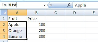
- Select the list that you want to use (it could also be from the table array you use for VLookup or HLookup. If it is, just select the list excluding the header which is the column one for VLookup table array or row one for HLookup table array). It is best if you can first sort your list in ascending order because the list taken in data validation will follow your actual list without sorting them for you.
- With the list selected, click in the name box located to the left of the formula bar and type a name (the name has to be unique and shouldn't be separated if it consists of more than one word) and then press Enter.
- Return to the other spreadsheet and select the cell(s) you want to create combo box.
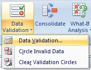
- With the cell(s) selected, go to Data tab and select Data Validation from Data Tools group (for Excel 2003 or earlier, go to Data menu and select Validation...).
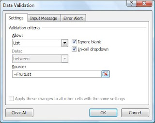
- On the Data Validation dialog box, go to Settings tab.
- Type the name you have given for the list in step 2, starting with the equal sign (=) in the Source field (I used FruitList for my example).


You can combine the usage of this combo box with any lookup function or use it alone.
- MRBAR


No comments:
Post a Comment